Identify faces in a video or live shot and recognize if they are wearing a mask: easy with the “raspberry”.
The spread of COVID-19 has created a global health crisis that has had a profound impact on humanity, the way we perceive our spaces and our daily lives. As of December 2019, we have witnessed the spread of this “acute respiratory syndrome” commonly referred to as coronavirus (SARS-CoV-2) that still has no cure and that forces us to defend ourselves from contagion by taking those precautions that have now become part of everyday life: wearing a surgical mask or better yet FFP2, disinfecting your hands after touching objects and places touched by others, maintaining a certain distance between people and avoiding leaving the house if you have a fever.
The use of the mask is now a necessary part of the rules for access to places frequented by the public and compliance with the requirement is the responsibility of the manager, who may do so when the flow of people allows it, but in places where the flow is greater and uncontrolled, such as a supermarket, a station, an airport, the obstacle can be overcome through artificial vision.
In this article we will explain how to do it using Raspberry Pi, which has all the necessary resources and which can be integrated into a compact stand-alone system to be placed on the gates of the places to be monitored. To do this, first of all we need to get an operating system in which all the stable libraries and frameworks are present; then it is essential to be able to have some algorithm to recognize a person within a series / sequence of images and more in detail their face; and finally a way to be able to distinguish between the various faces who has the personal protective device and who does not.
In this project we will involve artificial vision, also called Computer Vision (CV), that is the set of processes that allow to identify the content of images, but also artificial intelligence, which aims to recreate the human learning in computers.
Language
The programming language used is Python: object-oriented, it can be used for many types of software development because of its ease and integration with other types of languages. Clear and powerful, it is comparable to Java or Perl and like these uses an elegant syntax allowing you to easily read scripts and then create complex projects without sacrificing maintainability.
Today, according to several surveys, it is used by as much as 84% of developers as their primary programming language.
As far as the fields are concerned, among the most used we find Data Analysis and Web Development, but not only: other fields such as Machine learning, Computer graphics and Game development are starting to emerge.
The most used version is 3.6 and it is often used with IDE/Editor like PyCharm Professional/Community Edition or VS Code.
Given the small number of lines that we are going to write is recommended to install an editor only if you are a beginner, otherwise the pre-installed Nano or Text Editor are more than sufficient.
Although it is not as optimized as C++, especially with regard to the use of RAM and processor, it was chosen because it is open source, with a very large number of libraries also available at no additional cost and portable to any type of OS platform (Linux, Mac, Windows).
In our case in fact it will run on Raspbian, OS based on the official Debian releases adapted for an ARM architecture, but could easily be run on Windows without having to make many changes.
Our hardware
The recommended hardware for this project is 8GB Raspberry Pi 4, so you have a minimum of RAM available and also an updated system that can also support more audio and video processing. Based on an ARM processor, it offers performance comparable to an entry-level pc but can also handle 4k video streams. It also offers many pins, both of 3.3V power supply, and to interface peripherals, relays or sensors of different nature and manageable safely at the level of Python or C++ code through a set of libraries made available by the manufacturer.
To accompany this we are going to use a 5MP PI camera rev 1.3, which will be connected directly to the Raspberry Pi through the CSI connector. This module can offer a clear and crisp image with a resolution of 5MP or record video at 1,080p with 30 fps.
The sensor installed on the module has a 15-pin Ribbon connector and through the serial connection with the CSI connector offers an excellent data transfer speed, making this instrument particularly suitable for projects in the embedded / mobile field (Fig. 1).
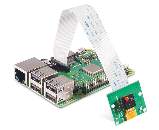
Fig. 1
System configuration
We are now going to install the operating system inside the Raspberry PI, which requires a microSD card with at least 16/32GB, Raspberry Pi Imager software and the zipper file with the actual operating system image. For the last two, the reference site is the official one: in the first section we will see imager, that is the tool with which to create a bootable SD-card able to start the device. Further on, always within the site, we find the zipper instead that we are going to upload, we report the direct link.
Once installed the imager, open it, insert our SD-card, and click CHOOSE OS.
Here select the last item or Custom OS and then choose the zipper downloaded earlier.
Then click on CHOOSE SD CARD and select the drive on which we want to restore the operating system and finally WRITE.
After a few moments we will have our SD card and we will be ready to start with our device.
You can use the preconfigured image rpi_32bit_facemaskdetector.zip in which are already present all the libraries and modules to be able to use the programs correctly.
In this case the credentials to access it are: user pi and password 12345678.
Insert the card into the Raspberry Pi reader, connect it to a network with internet access and turn it on. Once you have followed the first indications on general settings such as password, network etc, go into the settings, clicking on the icon of the raspberry in the upper left corner and choose Preferences>Configuration Raspberry Pi (Fig. 2): a screen like the one shown in Fig. 3 will appear and here click on Interfaces and enable the first two items, or Camera and SSH. The first for obvious reasons, in case we wanted to use an external PI camera module, while the second to connect remotely to the machine through tools such as Putty or WinSCP.

Fig. 2

Fig. 3
We close the menu by clicking OK and we will be asked to restart the system: let’s proceed. At reboot we open a terminal and always to be able to reach the machine remotely we install the remote desktop by typing:
sudo apt-get install xrdp -y
sudo apt-get update
sudo apt-get upgrade
Now we have all the tools to reach the machine remotely and then we can leave the monitor behind and act directly from our PC, the choice is yours. Let’s install now the two frameworks essential for any project of artificial vision and machine learning: OpenCV and Tensorflow. OpenCV is a library and a set of algorithms written in C for streaming and real-time image/video manipulation for computer vision available for all OS platforms. It allows the processing of images in a simple way, managing them as arrays of pixels. It allows us to perform the basic process of computer vision, i.e. Image processing, going to modify/improve images or sequences of images (video). It is widely used in science and research and can be used in different sectors: quality control, research, defense and many others.
With a few lines of code it is possible to recognize people in a photo, automatically read license plates, etc. All actions that would otherwise be very complicated to implement and integrate into larger projects.
In the case of embedded devices like this, the installation cannot be launched with a single command, but to have a precise control of the version we should install it starting directly from the sources.
To do this, open the terminal again and from the prompt pi@raspberrypi: ~ $ type the commands shown in sequence in Listing 1. These will allow us to install all those system components that will make us autonomous in compiling the sources and perform the installation.
Listing 1
sudo apt-get install build-essential cmake git unzip pkg-config -y
sudo apt-get install libjpeg-dev libpng-dev libtiff-dev -y
sudo apt-get install libavcodec-dev libavformat-dev libswscale-dev -y
sudo apt-get install libgtk2.0-dev libcanberra-gtk* -y
sudo apt-get install libxvidcore-dev libx264-dev libgtk-3-dev -y
sudo apt-get install python3-dev python3-numpy python3-pip -y
sudo apt-get install python-dev python-numpy -y
sudo apt-get install libtbb2 libtbb-dev libdc1394-22-dev -y
sudo apt-get install libv4l-dev v4l-utils -y
sudo apt-get install libjasper-dev libopenblas-dev libatlas-base-dev libblas-dev -y
sudo apt-get install liblapack-dev gfortran -y
sudo apt-get install gcc-arm* -y
sudo apt-get install protobuf-compiler -y
Let’s download the sources and decompress them using the following commands:
cd ~
wget -O opencv.zip https://github.com/opencv/opencv/archive/4.2.0.zip
wget -O opencv_contrib.zip https://github.com/opencv/opencv_contrib/archive/4.2.0.zip
unzip opencv.zip
unzip opencv_contrib.zip
mv opencv-4.2.0 opencv
mv opencv_contrib-4.2.0 opencv_contrib
Now let’s install the virtual environment where we can compile without damaging or altering the dependencies of the entire operating system, using the commands:
sudo pip3 install virtualenv
sudo pip3 install virtualenvwrapper
echo “export VIRTUALENVWRAPPER_PYTHON=/usr/bin/python3.7” >> ~/.bashrc
echo “export WORKON_HOME=$HOME/.virtualenvs” >> ~/.bashrc
echo “source /usr/local/bin/virtualenvwrapper.sh” >> ~/.bashrc
source ~/.bashrc
Finally we enter this test environment and compile the sources (as we see in Fig. 4) and verify that the compilation continues correctly (Fig. 5).

Fig. 4
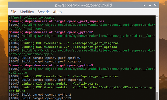
Fig. 5
Compilation times may vary depending on the machine we are working on: in our case we used a Raspberry Pi 4 with 8 GB of RAM and it took about half an hour.
Now we install the compiled file with the following commands:
sudo make install
sudo ldconfig
sudo apt-get update
cd ~
rm opencv.zip
rm opencv_contrib.zip
We close the terminal we are working on and open a new window in which we will type these last lines:
cd ~/.virtualenvs/cv420/lib/python3.7/site-packages
ln -s /usr/local/lib/python3.7/site-packages/cv2/python-3.7/cv2.cpython-37m-arm-linux-gnueabihf.so
cd ~
cd ~/opencv/build/lib/python3
sudo cp cv2.cpython-37m-arm-linux-gnueabihf.so /usr/local/lib/python3.7/dist-packages/cv2.so
cd ~
Once we’ve finished installing the first of the two macro libraries we move on to the second Tensorflow.
This one, a reference for machine learning, allows beginners and experts to easily create models for desktops, mobile devices, web and cloud. It will be used to create the model, i.e. a structure based on samples specially trained to discriminate various conditions, and then to use it within the algorithm, so that it can recognize faces and, most importantly, whether they are wearing protective gear or not.
Still on the terminal we type these commands to install some prerequisites:
sudo apt-get install libhdf5-dev libc-ares-dev libeigen3-dev -y
sudo apt-get install libatomic1 libatlas-base-dev -y
sudo pip3 install keras_applications==1.0.8 –no-deps
sudo pip3 install keras_preprocessing==1.0.5 –no-deps
sudo pip3 install h5py
sudo pip3 install keras_applications==1.0.8 –no-deps
sudo pip3 install keras_preprocessing==1.0.5 –no-deps
sudo pip3 install “h5py<3.0”
sudo pip3 install -U –user six wheel mock
Listing 2
mkvirtualenv cv420
pip3 install numpy
cd opencv
mkdir build
cd build
cmake -D CMAKE_BUILD_TYPE=RELEASE         -D CMAKE_INSTALL_PREFIX=/usr/local         -D OPENCV_EXTRA_MODULES_PATH=~/opencv_contrib/modules         -D ENABLE_NEON=ON         -D ENABLE_VFPV3=ON         -D WITH_OPENMP=ON         -D BUILD_TIFF=ON         -D WITH_FFMPEG=ON         -D WITH_GSTREAMER=ON         -D WITH_TBB=ON         -D BUILD_TBB=ON         -D BUILD_TESTS=OFF         -D WITH_EIGEN=OFF         -D WITH_V4L=ON         -D WITH_LIBV4L=ON         -D WITH_QT=OFF         -D WITH_VTK=OFF         -D OPENCV_EXTRA_EXE_LINKER_FLAGS=-latomic         -D OPENCV_ENABLE_NONFREE=ON         -D INSTALL_C_EXAMPLES=OFF         -D INSTALL_PYTHON_EXAMPLES=OFF         -D BUILD_NEW_PYTHON_SUPPORT=ON         -D BUILD_opencv_python3=TRUE         -D OPENCV_GENERATE_PKGCONFIG=ON         -D BUILD_EXAMPLES=OFF ..
make -j4
Now we download and install version 1.15.2 of the library dedicated to our ARM architecture, using the command:
wget https://github.com/Qengineering/Tensorflow-Raspberry-Pi/raw/master/tensorflow-1.15.2-cp37-cp37m-linux_armv7l.whl
sudo -H pip3 install tensorflow-1.15.2-cp37-cp37m-linux_armv7l.whl
sudo reboot
After the reboot, we install the latest libraries in order to properly run all the prepared Python scripts:
pip3 install keras==2.3.1
pip3 install imutils==0.5.3
pip3 install numpy==1.18.2
pip3 install matplotlib==3.2.1
pip3 install argparse==1.1
pip3 install scipy==1.4.1
pip3 install scikit-learn==0.23.1
pip3 install pillow==7.2.0
pip3 install “picamera[array]”
sudo apt-get install alsa-utils mplayer -y
sudo apt-get install festival –y
and download the Python sources using the following commands:
git clone https://github.com/danisk89/RiconoscimentoMascherinaPythonOpenCV.git
cd RiconoscimentoMascherinaPythonOpenCV
Model
As a first step we are going to implement a series of scripts in Python so that we can train one of our datasets using Keras and TensorFlow. The latter are the open source libraries of reference for machine learning of neural networks. While the latter we have already discussed extensively the former we can say that, written in Python too, allows a rapid prototyping of deep neural networks and focuses on ease of use, modularity and extensibility. In phase 0 we are going to build a model capable of determining whether or not the framed subject(s) have a mask as a personal protective device.
For simplicity and speed, the aforementioned model is already present in the folder and pre-trained, but for completeness the flow will be analyzed starting from here, which is useful if you want to make changes or expand the dataset with more current images and maybe add false positives for example through the use of bandanas or scarves.
To do this we would need a dataset, that is a series of images classified and divided into two macro groups: with mask or without mask.
In our case the above mentioned dataset (https://drive.google.com/drive/folders/1XDte2DL2Mf_hw4NsmGst7QtYoU7sMBVG?usp=sharing) consta di 3835 foto suddivise in 1919 del primo tipo e 1916 del secondo, che dovrà essere preso in esame dallo script Python train_mask_detector.py.
ap = argparse.ArgumentParser()
ap.add_argument(“-d”, “–dataset”, required=True,
help=”path to input dataset”)
ap.add_argument(“-p”, “–plot”, type=str, default=”plot.png”,
help=”path to output loss/accuracy plot”)
ap.add_argument(“-m”, “–model”, type=str,
default=”mask_detector.model”,
help=”path to output face mask detector model”)
args = vars(ap.parse_args())
INIT_LR = 1e-4
EPOCHS = 20
BS = 32
In the initial part we find the initialization of some constants as for example the file path .model in output from the training, the path of the file where the graphical report of the learning will be printed, the initial index of learning, the epochs, that is the number of presentations to the network of all the patterns of our training set and the dimension of the batch, that is the number of samples that will be propagated through the network.
imagePaths = list(paths.list_images(args[“dataset”]))
data = []
labels = []
for imagePath in imagePaths:
label = imagePath.split(os.path.sep)[-2]
image = load_img(imagePath, target_size=(224, 224))
image = img_to_array(image)
image = preprocess_input(image)
data.append(image)
labels.append(label)
data = np.array(data, dtype=”float32”)
labels = np.array(labels)
lb = LabelBinarizer()
labels = lb.fit_transform(labels)
labels = to_categorical(labels)
Next we find classification, subdivision of images and labels.
(trainX, testX, trainY, testY) = train_test_split(data, labels,
test_size=0.20, stratify=labels, random_state=42)
aug = ImageDataGenerator(
rotation_range=20,
zoom_range=0.15,
width_shift_range=0.2,
height_shift_range=0.2,
shear_range=0.15,
horizontal_flip=True,
fill_mode=”nearest”)
baseModel = MobileNetV2(weights=”imagenet”, include_top=False,
input_tensor=Input(shape=(224, 224, 3)))
headModel = baseModel.output
headModel = AveragePooling2D(pool_size=(7, 7))(headModel)
headModel = Flatten(name=”flatten”)(headModel)
headModel = Dense(128, activation=”relu”)(headModel)
headModel = Dropout(0.5)(headModel)
headModel = Dense(2, activation=”softmax”)(headModel)
model = Model(inputs=baseModel.input, outputs=headModel)
for layer in baseModel.layers:
layer.trainable = False
print(“[INFO] compiling model…”)
opt = Adam(lr=INIT_LR, decay=INIT_LR / EPOCHS)
model.compile(loss=”binary_crossentropy”, optimizer=opt,
metrics=[“accuracy”])
print(“[INFO] training head…”)
H = model.fit(
aug.flow(trainX, trainY, batch_size=BS),
steps_per_epoch=len(trainX) // BS,
validation_data=(testX, testY),
validation_steps=len(testX) // BS,
epochs=EPOCHS)
Now let’s load the MobileNetV2 network and insert it in the methods provided by the two open source libraries (mentioned at the beginning).
These last ones will give in output a model with which we will go to examine its decisional ability.
The MobileNetV2 is a convolutional neural network architecture whose purpose is to be very optimized to work properly on mobile devices. The commands needed are.
print(“[INFO] evaluating network…”)
predIdxs = model.predict(testX, batch_size=BS)
predIdxs = np.argmax(predIdxs, axis=1)
We have thus obtained the model in the form of a file that we are going to load inside our algorithm (Fig. 6).

Fig. 6
Algorithm
Once we have obtained the model responsible for determining the prediction with/without mask, let’s focus on how to easily acquire and process an image through the OpenCV library.
The first step is then to extract from that an image that can be processed:
import imutils
import time
import os
import cv2
import numpy as np
..
image = cv2.imread(Percorso dove trovare la foto/la foto)
With a disk image it’s very easy, but with a video it’s just as easy, since each video can be viewed as a series of images, of frames.
Now it will be sufficient to insert a while loop in which we will look at the state of the video and read frame by frame:
import imutils
import time
import os
import cv2
import numpy as np
…
cap = cv2.VideoCapture(Percorso dove trovare il video/il video)
if (cap.isOpened()== False):
print(“Error opening video stream or file”)
while(cap.isOpened()):
ret, frame = cap.read()
…
cv2.imshow(‘Frame’,frame)
Finally, we arrive at the most suitable configuration for our goal, which is to integrate the camera sensor as well:
from picamera.array import PiRGBArray
from picamera import PiCamera
import imutils
import time
import os
import cv2
import numpy as np
…
camera = PiCamera()
camera.resolution = (640, 480)
camera.framerate = 32
rawCapture = PiRGBArray(camera, size=(640, 480))
for frame in camera.capture_continuous(rawCapture, format=”bgr”, use_video_port=True):
frame = frame.array
…
cv2.imshow(‘Frame’,frame)
The extrapolated frame can also be scaled (reduced or enlarged) as needed.
After this phase of introduction to the library for video manipulation we begin to build the key algorithm to make the best use of our decision model.
To do this, as we did before, we load all the constants that are essential for the success of the work:
ap = argparse.ArgumentParser()
ap.add_argument(“-f”, “–face”, type=str,
default=”face_detector”,
help=”path to face detector model directory”)
ap.add_argument(“-m”, “–model”, type=str,
default=”mask_detector.model”,
help=”path to trained face mask detector model”)
ap.add_argument(“-c”, “–confidence”, type=float, default=0.5,
help=”minimum probability to filter weak detections”)
args = vars(ap.parse_args())
print(“[INFO] loading face detector model…”)
prototxtPath = os.path.sep.join([args[“face”], “deploy.prototxt”])
weightsPath = os.path.sep.join([args[“face”],
“res10_300x300_ssd_iter_140000.caffemodel”])
faceNet = cv2.dnn.readNet(prototxtPath, weightsPath)
print(“[INFO] loading face mask detector model…”)
maskNet = load_model(args[“model”])
As you can see, we have also brought in another model: this is essential to understand and isolate the various faces within the frame which will then be subjected to the analysis of our model. Pre-trained with Caffe, a well-known Deep Learning framework developed by Berkeley AI Research, our Artificial Intelligence model offers almost perfect face identification. This step can also be addressed through the Haar method, which is an effective object detection method proposed by Paul Viola and Michael Jones in their article “Rapid Object Detection Using an Enhanced Cascade of Simple Features” in 2001. It is a machine learning based approach where the waterfall function is trained by many positive and negative images. Once our models have been loaded, let’s manipulate the image by creating a 300×300 frame to identify the various faces in the scene.
(h, w) = frame.shape[:2]
blob = cv2.dnn.blobFromImage(frame, 1.0, (300, 300),
(104.0, 177.0, 123.0))
faceNet.setInput(blob)
detections = faceNet.forward()
For each face we suspect, we will analyze if the attributed value is higher than the threshold and only in this case we will perform the ROI of the face with the model to determine if the subject is with or without mask.
A ROI allows us to operate on a rectangular set of the image, for this reason it is very used especially to delineate those that are the primary markers such as eyes, nose and mouth.
for i in range(0, detections.shape[2]):
confidence = detections[0, 0, i, 2]
if confidence > args[“confidence”]:
box = detections[0, 0, i, 3:7] * np.array([w, h, w, h])
(startX, startY, endX, endY) = box.astype(“int”)
(startX, startY) = (max(0, startX), max(0, startY))
(endX, endY) = (min(w – 1, endX), min(h – 1, endY))
face = frame[startY:endY, startX:endX]
face = cv2.cvtColor(face, cv2.COLOR_BGR2RGB)
face = cv2.resize(face, (224, 224))
face = img_to_array(face)
face = preprocess_input(face)
faces.append(face)
locs.append((startX, startY, endX, endY))
And finally, once we have made sure we have faces, let’s use the model to discriminate whether or not they have the personal protective device and we report everything in a variable.
faces = np.array(faces, dtype=”float32”)
preds = maskNet.predict(faces, batch_size=32)
At this point we have everything: in the variable locs we find the X, Y coordinates of where the faces are and their size, while in the variable preds we can see if these faces respect the security measures imposed. However, at the video level we don’t have any proof of what we have found, so we need a further step to mark inside the frame what are the faces and their attributes. For this reason, for each face we are going to make a new cycle in which we are going to modify the frame by adding rectangles and overlays where the coordinates extrapolated in the previous point indicate a face.
for (box, pred) in zip(locs, preds):
(startX, startY, endX, endY) = box
(mask, withoutMask) = pred
label = “Mask” if mask > 0.85 else “No Mask”
color = (0, 255, 0) if label == “Mask” else (0, 0, 255)
label = “{}: {:.2f}%”.format(label, max(mask, withoutMask) * 100)
if label==”Mask”:
faceMask=faceMask+1
else:
faceNoMask=faceNoMask+1
cv2.putText(frame, label, (startX, startY – 10),
cv2.FONT_HERSHEY_SIMPLEX, 0.45, color, 2)
cv2.rectangle(frame, (startX, startY), (endX, endY), color, 2)
Regarding the fourth line, theoretically it would be possible to discriminate also with a condition like mask>withoutMask, but it is very light and fragile, so it is preferable to compare it with a percentage value.
It’s also possible to add a further signaling of the results: the audio channel; in fact, as you can see from the previous portion of code, it’s possible to count the faces and then insert a signaling different from the video only. In particular, it is preferable a thread that deals with this aspect, in order not to burden the already difficult task of discerning and showing on screen. This thread can also be invoked maybe once every 10 frames in order to have the possibility to collect several frames on which to base its reporting.
if index==10 :
_thread.start_new_thread(speakTTS, (faceNoMask,faceMask,1))
index = 0
index = index + 1
def speakTTS(faceNoMask,a,b):
if faceNoMask == 0 :
if a==0 :
os.system(‘echo “” | festival –tts’)
else:
if a==1 :
os.system(‘echo “Pass the check” | festival –tts’)
else:
os.system(‘echo “All the ‘+str(a)+’ persons pass the check” | festival –tts’)
else:
if faceNoMask == 1 :
os.system(‘echo “There is ‘+str(faceNoMask)+’ person without mask protection” | festival –tts’)
else:
os.system(‘echo “There are ‘+str(faceNoMask)+’ persons without mask protection” | festival –tts’)
To execute our algorithm we open a new terminal window and issue the command:
python3 cam_video.py
The result obtained will be like that in Fig. 7, with the face in the green box if the system has detected the mask and in red in the opposite case; all in real-time in order to evaluate each situation in the shortest possible time without creating long files. The system justifies the outcome with an attached indication about the probability that the situation shown is the true one, i.e. with Mask in green and the percentage of probability if it believes that the face has the mask, or No mask in red and its percentage of probability that the face framed is without the mask.
In short, we are given not only a verdict, but also a way to judge how much the system is doing the right thing. And it is not so small…
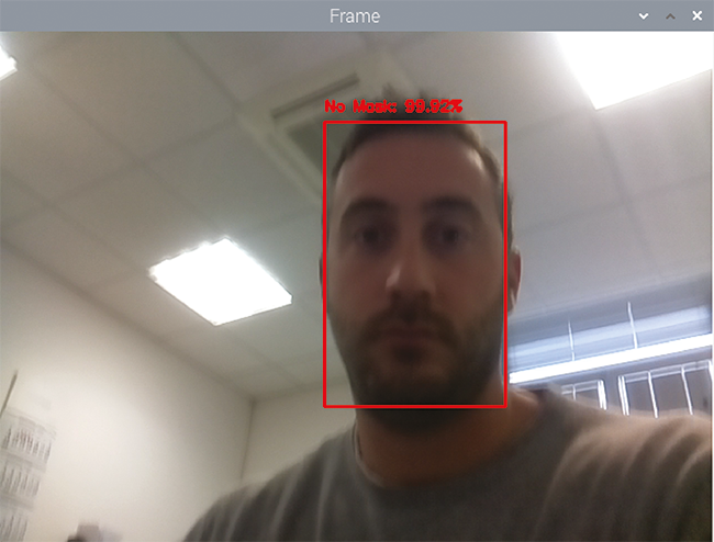
Fig. 7
Conclusions
The activity obviously does not stop here: in fact we could have two further implementations that could bring this educational project to a much higher level. First, we can make the output video stream completely fluid and above all normalize the times when we have very dense scenes, perhaps through a parallelization of face tracking through different threads properly semaphorised.
We would like to emphasize the “appropriately semaphored” aspect since all workers will then have to converge in the global prediction function, so they will have to do the work and wait for each other in order to provide a single output response. With few faces this implementation does not improve, if at all, the video output, while in case of 10/15 faces it radically changes the timing.
Another realization could be to migrate this work in a different operating system like Ubuntu Server, always on Raspberry Pi.
In this case you wouldn’t have any UI on which to see faces and recognition but this would only work as a smart camera.
Once the data is processed, the camera could have a system of pushing the information into a cloud from which it would be distributed to the connected units; this means that, perhaps, through an app on a smartphone we can see in real time the video processed by my device and have information about faces and whether or not they are wearing a mask.
It will then be the app’s task to show the video stream, as in our version, with faces marked by red and green squares; or we can receive only the basic information, however in this case more elements would be involved than in a basic situation like the one developed in this article: in addition to the ability to develop an app (which requires skills from the Android or iOS world) you should have knowledge of light protocols of data/video transmission such as MQTT or RTMP and know how to set up a server to receive and retransmit data.
Certainly the task is challenging but stimulating and can be an opportunity to acquire new skills.
From Open Store