LED MATRIX: giant & stand-alone panels

• Tweet
• Pin It

You already had the chance to see – and we hope, to try – our modular system for RGB LED matrix displays: LED Matrix (that’s the name) is a solution based on RGB LED matrices, that may be easily acquired (and at an affordable price) since they were born in the Maker world. We manage it by means of a controller board of the same name, that is an extremely powerful one since it’s the FPGA Spartan 6 by Xilinx, and it does not limit itself to the matrix management (that you could see in the previous installments) but – thanks to a specific firmware (bitstream ones, given that we are talking about FPGA…) – it may drive displays having a greater size, or that may carry out other tasks (that we will describe later).

The applications we proposed in the past  concern 32×32, 64×32 or 128×32 pixel (LED) matrices: and they are based on a free firmware, supplied with the board. There are also  paid extensions of the LED Matrix board, based on a paid firmware and they enable, as an example, to manage matrices having a bigger size, and to do that autonomously from PC, in the stand-alone mode. The latter is particularly valuable when you have to install a display in a place that is not easily accessible, or where you have to operate by continuously reproducing the same animation.

In these pages, we will describe the SD-Card section (that we omitted until now from the circuit diagram analysis) and the one that enables the “cascading”, needed in order to drive large matrices.

But let’s proceed step by step and first deal with the variations needed for controlling a display having a size that is greater than the one allowed by the board’s free version.

Extended Matrices

A single LED Matrix controller board may drive RGB LED matrix displays up to a maximum of 64×64 LEDs, and that are therefore composed of four 32×32 modules, arranged so to form a quadrilateral, and connected in cascade among them and to the board’s outputs. But the system enables the management of panels that are extended up to Jinx’s limit (that’s the viewing software for Windows,) which is 48,000 pixels, a limit that goes well beyond 64×64. However, because of the limits of the Spartan 6 capabilities, it is not possible to control of all of them with a single unit, otherwise the refresh will be slowed down, to the detriment of the video playback quality.

In this case, one would resort to the cascading, that is to say, to a particular configuration that enables the connection in cascade of more units, so to entrust the control of a pixel block to each one of them.

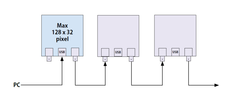
In the said mode, the board is connected to the computer and repeats the whole data stream towards the following one, by means of the BNC connection (that we omitted during the analysis of the circuit diagram, but we will soon deal with it); the board receiving the stream through the input BNC will repeat it on the output one. The following one will do the same to the following.

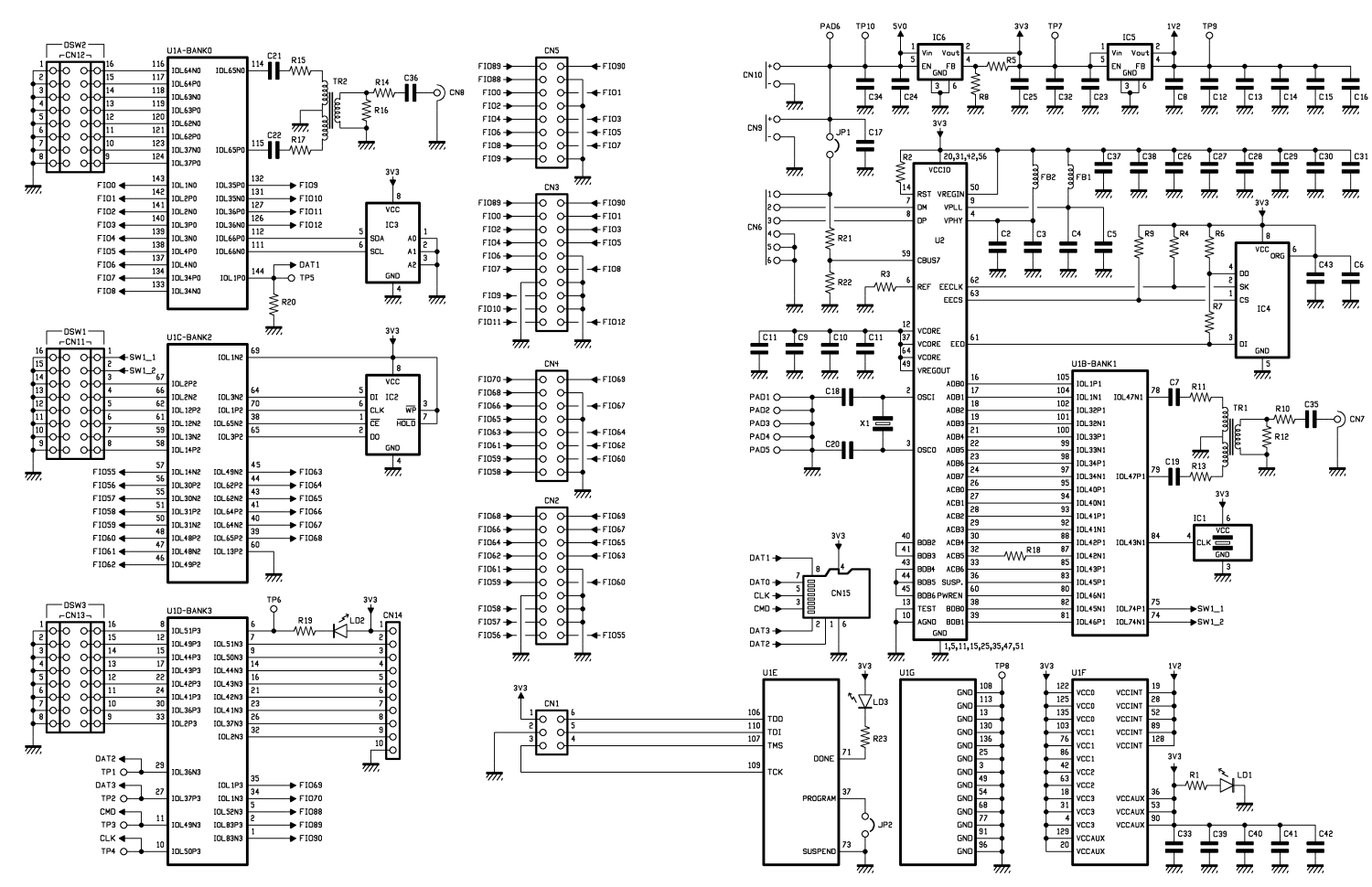
In the said mode, the FPGA firmware decides how to subdivide the stream’s pieces of data, on the basis of the configuration that is loaded by means of the terminal program; in other words, it is by means of the terminal that we decide and tell how the display is formed (we will later see the commands to give) to the board that is connected via USB; and at this stage each one displays only its part of data and repeats the whole stream on BNC. The BNC connectors are signed CN7 and CN8; they are respectively input and output. The board that comes soon after that one is connected in cascade via the other BNC and uses only the pieces of data that concern it, while it repeats the stream on BNC; it goes on like this till the last board.

A peculiarity of the FPGA lines that are repeated on the BNCs is that they are set so to operate in differential mode and are uncoupled on the demoboard by means of signal transformers (TR1 and TR2) with centre tapped secondary winding, that enable the galvanic isolation, thus ensuring a greater immunity to electrical noises.

Their processing will then be carried out by the FPGA blocks, that will be selected from time to time by the application’s firmware. Please notice that the term “differential” concerns the internal side of the board and not the BNC: in fact, the inputs are unbalanced at the BNC (that is to say, they are connected to a contact with respect to ground), while from the side of the FPGA they are balanced, that is to say, they refer to two I/Os. Each BNC is uncoupled by means of a capacitor in series to the signal wire, so that if some devices that have a DC polarisation are connected to the demoboard, the transformer does not act as load; moreover there is a 75 ohm resistor in series to each BNC, and it adjusts the input impedance to such a value. From the internal side, the transformer with centre tapped secondary winding (connected to ground) supplies two signals in phase opposition, each one of them – by means of R/C dipoles series (so to uncouple and stabilise the impedance) – is connected to a pair of FPGA’s I/Os.

A peculiarity of the cascading mode is that it enables the extension of the PC-Matrix connection beyond the maximum of 5 metres of the USB standard connection. Typically, the common USB 2.0 cables are capable of ensuring a maximum speed of 480 Mbit/s (USB 2.0 Full Speed) only with lengths of about two metres, even though the maximum distance supported is, in theory, 5 metres. This is due to the crosstalk and to the low or missing shielding of the cheap “consumer” cables, that moreover weaken and distort the signal, beyond a certain distance, thus forcing the USB controllers to decrease the speed.

Beyond this distance it would not be possible, therefore, to command the RGB matrix from the PC, but our LED Matrix has an ace up the sleeve, that consists in using the BNC connection that – since it is based on differential lines – ensures a very high immunity to noises, also by virtue of the low impedance of the connection, that has a typical value of 75 ohm (that’s not a case it requires a RG59 75 ohm cable). Therefore, if the PC is farther than the 5 metres allowed by the USB, we just need to connect it to a first LED Matrix controller board that in this case would act as a repeater, and then get the right BNC signal (CN8) and send it to the display block, at the BNC input (CN7) of the first controller board (that is to say, the one that drives the matrix that has been chosen first in the order). The firmware fully supports such a mode, meaning that it repeats everything arriving on USB, regardless of the fact that the board connected to the PC drives a part of the display or not. After that, the first board of the visualizer will analyse the stream incoming on its CN7 and will process the part falling within its competence, and repeat the stream on its CN8 (as we already explained).

In the said mode it is possible to connect the panel and therefore the first board in the chain, even at a distance beyond 50 metres, provided that the coaxial cable is a good quality one.

SD-Card Section

Let’s move on now to the playback mode from SD-Card, that is the stand-alone one, since you do not need to connect any PC. As for it, everything we said until now – with regard to the array modularity and the display support – is still valid; the only difference is that the cascading is not supported. In the said operating mode, the firmware searches in the SD-Card inserted in the controller board for the file to be played; the controller board has been opportunely instructed by the specific commands given from terminal, so to activate the said functioning mode. The file has to be the one generated by Jinx, by means of the dedicated function and the corresponding menu commands (that we will later describe).

As regards the concerned hardware, it’s time for a digression: in order to speed up the access to the Card, from which the FPGA firmware enables to execute the file containing the data needed in order to build the pictures in real time, we used faster mode, that is not the classic SPI (the one we were used to, thanks to Arduino and derivative boards, and that is used by the consumer microcontrollers); here we use the full-speed mode, and separate the pieces of data from the commands (that in the SPI-type buses travel on a single wire, on the other hand) and use as much as four bidirectional lines for reading and writing (they are DAT0, DAT1, DAT2, DAT3, and along them the pieces of data travel in packets that are then put back together at the right moment).

As regards the commands, we use the CMD channel and all the communications on DAT0÷DAT3 and CMD are seton the clock that the FPGA sends to the line of the same name. In the board, the SD-Card reader’s data channels (respectively DAT0, DAT1, DAT2, CD/DAT3) are connected to the FPGA’s lines, IO_L52P_3 (6), IO_LIP_HSWAPEN_0 (144), IO_L36N_3 (29), IO_L37P_3 (27); the SD-Card’s clock connects to IO_L50P_3 (pin 10) while the CMD channel goes to pin 11 (IO_L49N-3).  

With such a configuration, we manage to transfer data (if the Card we are using supports it) at a speed that may even reach 70 MB/s, and therefore 560 Mbps! That’s more than enough for the playback of files with animations, at the resolution that is envisaged by the biggest display supported by a board.

Unit configuration

Let’s move on now to the part you will probably be most interested into, that is to say, how to make up the modular panel; as hinted before, each board must be configured on the basis of the display it has to drive.

Therefore, the first thing to do is to decide and define the display architecture, and to remember that each LED Matrix controller drives two basic matrices that are connected in cascade by means of a flat-cable, and to use each one of the connectors it has, for the purpose (CN6 does the first part and CN5 the possible second one).

Therefore, if you have to drive a single block (16×32, 32×32, up to 16×64) you just need to connect it via CN4, while if you have to drive two, or anyway if you have to manage blocks that are composed of more than 32×64 pixels, you will also have to use CN5, with which to connect the second block.

This being said, it is the case to point out that we conventionally name a display block entrusted to a single LED Matrix controller as Tile (we will see how to carry out the configuration), the set of Tiles composing the whole display to be created is defined as an Array.

Please remember that when the Array counts more than one Tile, you will have to individually configure the controller boards, and to define for each of them their position inside the Array itself. Once it has been established how big is the Array, you will have to set the size of the single Tile, also on the basis of what you have available.

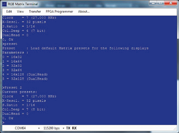
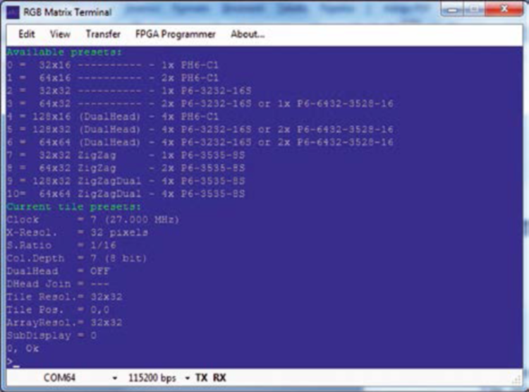
In order to configure the visualizer, as a first thing we have to launch the LED Matrix terminal, and after having chosen the virtual COM to which the board to be configured has been assigned, when at the command prompt (>) please type preset and press Tab: the screen will show the available options, having the Tile resolution (0=16×32, 1=16×64 ecc.) next to each numeric value of the parameter.

We now have to type preset, followed by the value identifying the Tile composition, that must be decided at the beginning, on the basis of the visualizers composition. As an example, if we want to create a 128×128 pixel panel – knowing that each board reaches a maximum of 128×32 LEDs – we will need four 128×32 Tiles, and therefore as many controller boards. Please remember that the 16×32 matrices may be connected only in a row, the 32×32 may be connected in a row or on a square, and the same goes for the 64×32 ones.

Let’s verify, for now, the current settings, by typing preset and Return; the screen will return the settings; while in there, at X-Resol. the Tile’s horizontal resolution is indicated. If different, let’s set the value we’re interested in – that is to say, 32×32 – and then give the preset 2 command: the screen will show the new situation, and will update the X-Resol. field.

By giving the Tileres command, followed by Return, you will be able to verify the Tile’s settings or to change them, if need be. It is needed, when writing the command, to leave a space between the comma and the y value, otherwise the command will not be executed and nothing is communicated from the terminal.

Once this has been done, the array size must be defined, therefore – and still from the terminal window – we will give the ArrayRes command, followed by Return. The screen will show the current resolution. By typing ArrayRes, followed by the x and y resolutions (that is to say, the number of horizontal and vertical pixels), you will set the array size. For example, as for our 128×128 pixel panel, we will type ArrayRes 128, 128 and press Return.

The last setting to be given is the one of the starting pixel (the one in the upper corner and on the left), that falls within the competence of the tile associated with the controller, in the full matrix (array): by giving the Tilepos x, y command, we define the first pixel, that in our case is 0, 0 for the first board (the one connected to the PC), 32, 0 for the second one, 0, 32 for the third one and 32, 32 for the fourth one shows the Tilepos setting.

Once this has been done, in order for the configuration to be permanent, we will have to type Save and to press the Return button.

At this stage, it is possible to assemble the system, but please keep in mind that the right BNC of the board that will be connected to the Personal Computer has be connected to the left one of the other board, by means of a RG59 coaxial cable (75 ohm) that has BNC connectors at the ends. After that, please power the LED matrix modules in parallel among them, by means of an adequate power supply, and cables having a section of 2.5 sq mm.

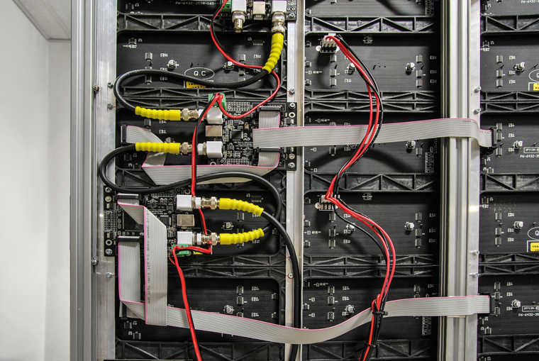
Figure shows our sample 128×128 pixel panel, that we created for our tests, and that is composed by four 128×32 Tiles, by two 5V switching power supplies (one for each half of the panel) and by four controller boards; you will see that each board drives the first 32×32 matrices via CN4, and the last two via CN5. Please refer to it, when taking the cue for your creations.

Download Terminal

Download BIN file

Setting Jinx

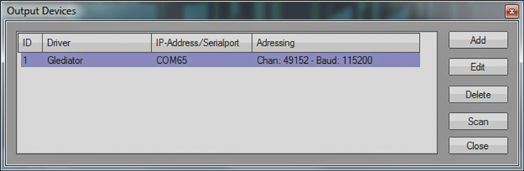
While in Jinx, you may manually configure the display structure or load a configuration file that was previously saved. As explained in the past installment, please proceed to the configuration of jinx, by means of the “setup->matrix options” menu, and configure the total panel size, then enter the “Setup->Output patch” menu and configure the whole panel by means of the “Fast patch” button. Finally, please enter the “Setup->Output devices” menu and configure the USB streaming interface you wish, by using the glediator protocol.

Once the whole has been configured, it will be possible to activate the streaming from the “Setup-Start output” menu.

Once the system has been configured, we strongly advise to save the jinx configuration from the “File-Save as” menu entry, so to easily recall it, when needed. Also, we would like to remind you that at the start, Jinx will automatically load the last configuration that was saved and used.

SD Configuration

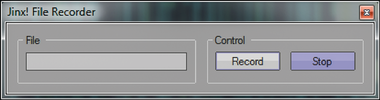
Let’s move on now to the configuration of the SD mode: this is actually the same, but when opening the terminal and selecting the command COM, the C:\> prompt will appear, so to indicate that in the board a mass memory unit was found. We would like to remind you that the stand-alone mode requires that in the LED Matrix controller board the SD-Card option has been purchased and enabled, otherwise the Card will be ignored. In order to create a file for the SD-Card in Jinx, it will be enough to press the F4 button (at any time), and a window will appear: it will ask for the file in which to save the animation. The recording starts by clicking on Record and by specifying the path and filename you wish to create; once the file has been defined and you have clicked on OK, the computer will start recording everything happening. Whenever you want to end the recording, please click on OK. The corresponding file will be saved in the .jnr format.

At this stage, please get your SD-Card, that must be FAT32 formatted, then insert it in the reader that is integrated to the computer (or connected via USB to the PC) and copy the file there, after that – with the controller turned off – please put it in the specific socket. Please turn on the controller and launch the terminal on PC: you will notice that the C:\> command prompt will appear.

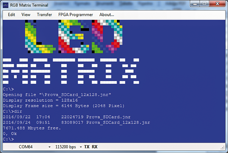
 As soon as the prompt appears, please type dir, so to see the files found  and then Play, followed by the name of the file you’re interested.

Please save the configuration by means of Save command; thus you will have created the file that, from now on, when turning on the controller board will be automatically executed, by visualizing the animation loaded in the SD-Card on the display (even with the PC being disconnected, and independently). The Play command, followed by the filename, and given from the terminal, is needed in order to carry out manual tests along with the unit connected to the computer. Please remember that in order to obtain the best performances as for the viewing speed (fluid animations), we advise you to use class 6 SD Cards, or even better, class 10 ones, given the high reproduction speed required.

VIDEO

From openstore

LED Matrix controller RGB

16×32 RGB LED panel

32×32 RGB LED panel

64×32 RGB LED panel

Cascading module enabling

Enable SD Card Module

Related Posts

• 

  Building a 3D Digital Clock with Arduino
  Building a 3D Digital Clock with Arduino
• 

  Creating a controller for Minecraft with realistic body movements using Arduino
  Creating a controller for Minecraft with realistic body movements using Arduino
• 

  Snowflake with Arduino
  Snowflake with Arduino
• 

  Holographic Christmas Tree
  Holographic Christmas Tree