Facial recognition with OpenCV4

• Tweet
• Pin It

 

Let’s experiment with the OpenCV 4 library in real-time face recognition and smile detection project.

In the article “Home automation with OpenCV 4” we have introduced the OpenCV 4 library for Raspberry Pi, which represents a powerful tool to realize applications in the field of image detection with a specific camera for Raspberry Pi.

On the same occasion, we explained how to install the OpenCV 4 library for the Raspbian platform and how you can use a Raspberry Pi board to create a simple motion recognition system by analyzing the images taken by the specific camera for the same board. Now let’s continue on the same trend by analyzing new features of the library with the aim of creating a facial recognition system capable of detecting a face, eyes and a smiling mouth; all in real-time.

In exposing this application project we will take for granted some things: for example that you have already set up the system based on Raspberry Pi and that you have run the OpenCV 4 installation, as explained in the Home Automation article with OpenCV 4 published in the issue No. 233. If you have not already done so, carefully follow the instructions of the article and proceed.

That said, we can start.

 

Haar Cascades

A technique used by OpenCV 4 for face detection is based on the so-called Haar Cascades. In other words, they are cascading classifications based on the Haar algorithm, named in honour of the Hungarian mathematician Alfréd Haar, famous for his studies at the beginning of the 1900s and to whom the Haar wavelet was recognized (see the in-depth section in this same page).

The Haar Cascades represents a very effective optical detection method for objects, proposed by Paul Viola and Michael Jones in their 2001 article “Rapid Object Detection using a Boosted Cascade of Simple Features”, which translated sounds like “Rapid detection of objects using cascades increased with simple features ”.

It is an approach to machine learning based on a cascade function that is “trained” by simple features. As we will explain shortly, Haar’s wavelet technique creates positive and negative boxes to be used as filters to be superimposed in sequence on an image, from whose interaction the necessary information is extracted to understand where a certain characteristic of the object is located. For example a face, eyes and mouth (Fig. 1).

 

Fig. 1

 

As you can see in the figure, the boxes that are obtained with the Haar wavelet are subdivided into three Features (a term that can be translated as “features”, but we will leave it in English because normally we use this slang term):

 

(a) Edge Features

(b) Line Features

(c) Four-rectangle Features

These features are applied in cascade and, initially, the algorithm requires many images of faces and images without faces.

This is the method to “train” the so-called classifier. For this purpose, the features of Haar are used, the application of which is shown in Fig. 2. It is easy to see how the Haar algorithm produces white and black rectangular boxes, through a square wave matrix.

It should be noted that the images to be processed must be transformed into grayscale if they are in colour. This is to facilitate the calculation with white and black boxes.

Subsequently, once the character of a face, eyes etc. have been found, the colour image can be reused.

 

Fig. 2

 

Each Feature is extracted from a single value, obtained by subtracting the sum of the pixels under the white rectangle from the sum of the pixels under the black rectangle. The boxes move quickly over the whole image and all the possible dimensions and positions of the face are used to calculate the features.

More than 160,000 features are required for a 24×24 pixel window. For each Feature calculation, you need to find the sum of the pixels under the black and white rectangles.

To solve this problem and how big the image to be processed, the calculations for a given pixel are reduced to an operation that involves only four pixels at a time, making it very fast.

Of all these features that are calculated, most are irrelevant. For example, if we look at Fig. 2, the top line shows two good features. The first selected Feature seems to focus on the property that the eye region is often darker than the region of the nose and cheeks.

The second Feature is based on the property that the eyes are darker than the nose. But the same windows applied to the cheeks or to any other place are irrelevant.

So, to select the best features from 160,000, an Adaboost algorithm was created, with which the best threshold for classifying faces is found. For the record, AdaBoost, short for Adaptive Boosting, is a meta-algorithm for automatic learning, formulated to be used in machine learning.

Obviously, during the Feature extraction operation, there will be errors or incorrect classifications, so the Features are selected with a minimum error rate to more accurately detect face images.

The process is not so simple: each image is given a weight equal to the beginning, after each classification, the weights of the wrong images are increased, then the same process is performed and new error rates and new weights are calculated.

The process continues until the required accuracy or minimum error rate is reached. The final classifier is a weighted sum of these “weak” classifiers. They are called weak because by themselves they cannot classify the image, but together with others, they form a strong classifier. Experience in the field tells us that even 200 Features provide detection with an accuracy of 95%.

The final configuration will have around 6,000 features and this reduction from 160,000 to 6,000 is a great advantage. As we shall see, all the classifier parameters (classifier) ​​are saved in files ready for use (pre-trained files).

 

Cascade of Classifiers

Despite the reduction to around 6,000 features, to reduce the time for the detection of a face, the concept of Cascade of Classifiers has been introduced.

Usually, in a frame most of the image is not a face, so the best method is to check if a region of the photo is not a face.

If it is not, this region is immediately discarded and is not processed again, to the advantage of optimizing resources and processing times. Instead, the regions in which there can be a face are processed to check and analyze possible areas of the face.

To achieve this, the Cascade of Classifiers concept instead of applying all the 6,000 features in a window, groups them into different stages of classifiers and then applied one by one. If a window fails the first stage, it is discarded and the remaining features are not considered. If instead it passes, the second phase of the Feature is applied and the process continues.

The window that passes all the phases is a region of the face.

This region is called ROI (Region of Interest) and will be the one that will be considered for a subsequent analysis.

 

Haar-cascade di OpenCV 4

OpenCV has a trainer and a detector. If you want to “train” the classifier to identify any object such as cars, planes, etc. you can use OpenCV to create one.

The full details cannot be treated (for brevity) in this article, but know that they are on the official OpenCV website, on the Cascade Classifier Training web page

(Https://docs.opencv.org/4.0.0/dc/d88/tutorial_traincascade.html).

Here we will deal only with the survey. OpenCV 4 already contains many pre-trained classifiers for the recognition of face, eyes, smiles, bodies, car plates etc. The relevant XML files are available in the opencv / data / haarcascades folder (at least, if you have correctly installed OpenCV).

 

Face and eye detection with OpenCV

Below we present a simple Python listing that can perform face and eye detection from a still image.

First, we need to load the XML classifiers required for face and eye detection:

haarcascade_frontalface_default.xml

haarcascade_eye.xml

 

The most curious will want to know what these XML files contain. Just to give an idea of ​​the structure, we will hasten that, in addition to the typical structure of an XML file, we can distinguish the tags related to the 24×24 pixel window and the weakClassifiers tags (weak classifiers).

Depending on the type of detection, there are almost 3,000 tags called internalNodes which are combined with as many tag rects and about 6,000 leafValues ​​tags. The numbers can refer to measurements and coordinates of the rectangles and to the threshold values ​​of the classification stages (stageThreshold).

Listing 1 shows an extract from the file haarcascade_frontalface_default.xml.

We recommend copying these XML classifiers from the / home / pi / opencv / data / haarcascades folder into a new folder; we called it face_eye_detect. In this folder, you also put a jpg image.

For our example, we used the image of the author, contained in the file “pier.jpg”.

Warning! Before starting to work with Python, remember to activate the “cv” virtual environment profile and open the Python idle with the following commands from the terminal, as shown in Fig. 3:

source ~/.profile

workon cv

python -m idlelib.idle

 

For details, we refer to the article “Home automation with OpenCV 4” published in the previous post.

Analyzing the listing in Python, we first import the necessary libraries:

 

import sys

import os

import numpy as np

import cv2 as cv

 

 

So, let’s create the face_cascade object with the classifiers obtained from importing the first XML file for face detection.

 

Fig. 3

 

Similarly, we create the eye_cascade object with the classifiers obtained from importing the second XML file for eye detection.

So, we load the jpg image to be analyzed and transform it into grayscale with the cv.COLOR_BGR2GRAY function.

The img object will contain the image information and the gray object those of the image transformed into grayscale.

Then proceed with the commands:

face_cascade = cv.CascadeClassifier(‘haarcascade_frontalface_default.xml’)

eye_cascade = cv.CascadeClassifier(‘haarcascade_eye.xml’)

img = cv.imread(‘pier.jpg’)

gray = cv.cvtColor(img, cv.COLOR_BGR2GRAY)

 

At this point, we can look for the face in the image using the function face_cascade.detectMultiScale (gray, 1.3, 5).

The for loop looks for a face within the faces object passing the x and y coordinates and the width and height w and h dimensions of the Feature.

If a face is found, its position will be highlighted with a blue rectangle, using the function cv.rectangle (img, (x, y), (x + w, y + h), (255,0,0), 2).

Once we get the face position, we can create a so-called ROI (Region of Interest) for the face and apply eye tracking on this ROI, since the eyes are always on the face.

With the same procedure, once the eyes are detected, they are highlighted with two green rectangles:

 

faces = face_cascade.detectMultiScale(gray, 1.3, 5)

for (x,y,w,h) in faces:

    cv.rectangle(img,(x,y),(x+w,y+h),(255,0,0),2)

    roi_gray = gray[y:y+h, x:x+w]

    roi_color = img[y:y+h, x:x+w]

 

    eyes = eye_cascade.detectMultiScale(roi_gray)

    for (ex,ey,ew,eh) in eyes:

        cv.rectangle(roi_color,(ex,ey),(ex+ew,ey+eh),(0,255,0),2)

 

Finally, a window is created with the instruction cv.imshow (‘img’, img) to display the result. The “img” window containing the result is visible in Fig. 4.

Once the window is closed, the program is terminated:

cv.imshow(‘img’,img)

cv.waitKey(0)

cv.destroyAllWindows()

 

Smile detection with OpenCV 4

Now let’s move on to a simple series of instructions to get the smile detection, done by analyzing a short video file.

To this end, the two classifiers will be needed:

haarcascade_frontalface_default.xml

haarcascade_smile.xml

 

Fig. 4

 

After loading the necessary libraries, the objects face_cascade and smile_cascade are created as explained above. The cv2.VideoCapture function allows you to load the movie. Our demo video is called ‘pier_smile.mp4’ and is that of a face at first serious and then smiling. The video capture resolution is 640×480 and the scale factor (sF) is 1.05.

 

import cv2

import numpy as np

import sys

 

face_cascade = cv2.CascadeClassifier(“haarcascade_frontalface_default.xml”)

smile_cascade = cv2.CascadeClassifier(“haarcascade_smile.xml”)

 

cap = cv2.VideoCapture(‘pier_smile.mp4’)

cap.set(3,640)

cap.set(4,480)

sF = 1.05   

 

The while loop analyzes all the frames of the video, transforming them into grayscale images, exactly as in the previous example. Please note that now the img object is a frame captured from time to time by the function cap.read ().

while (cap.isOpened()):

    ret, frame = cap.read()

    img = frame

    gray = cv2.cvtColor(frame, cv2.COLOR_BGR2GRAY)

 

The face_cascade.detectMultiScale function will look for the face in the video (better, in every frame) …

 

    faces = face_cascade.detectMultiScale(

        gray,

        scaleFactor= sF,

        minNeighbors=8,

        minSize=(55, 55),

        flags=cv2.CASCADE_SCALE_IMAGE

    )

 

… and, once found, will create a region of interest through the lines of code:

 

       for (x, y, w, h) in faces:

        roi_gray = gray[y:y+h, x:x+w]

        roi_color = frame[y:y+h, x:x+w]

 

The smile_cascade.detectMultiScale function will look for a smile inside the face …

       smile = smile_cascade.detectMultiScale(

            roi_gray,

            scaleFactor= 1.7,

            minNeighbors=22,

            minSize=(25, 25),

            flags=cv2.CASCADE_SCALE_IMAGE

            )

 

… and once found, will draw a rectangle around the smile, while in the terminal window will be printed “Found a smile”.

 

for (x, y, w, h) in smile:

        print(“Trovato un sorriso!”)

        cv2.rectangle(roi_color, (x, y), (x+w, y+h), (255, 0, 0), 1)

 

In the “Smile Detector” window you can see the result (Fig. 5). If you press the ESC key the program is terminated.

 

    cv2.imshow(‘Smile Detector’, frame)

    c = cv2.waitKey(7) % 0x100

    if c == 27:

        break

cap.release()

cv2.destroyAllWindows()

 

Fig. 5

 

Facial recognition in real time

The third experiment for face detection involves the use of a normal USB webcam.

As usual, the necessary libraries and the classifier haarcascade_frontalface_default.xml are imported at the beginning of the script.

With the cv2.VideoCapture (0) function seen above it is possible to directly capture the video of a USB webcam by passing parameter 0.

 

import cv2

import sys

cascade_path = “haarcascade_frontalface_default.xml”

face_cascade = cv2.CascadeClassifier(cascade_path)

video_capture = cv2.VideoCapture(0)

 

The while loop checks that a webcam is connected and then captures the frame by frame. As usual, all frames are converted to grayscale.

 

while True:

    if not video_capture.isOpened():

        print(‘Unable to load camera.’)

        pass

    ret, frame = video_capture.read()

    gray = cv2.cvtColor(frame, cv2.COLOR_BGR2GRAY)

 

The face_cascade.detectMultiScale function searches for a face in video streaming (better yet, in each frame) through the instructions:

 

    faces = face_cascade.detectMultiScale(

        gray,

        scaleFactor=1.1,

        minNeighbors=5,

        minSize=(30, 30)

    )

 

… and draw a rectangle around the face when it is found.

Keep in mind that with the parameter minSize = (30.30) it is possible to detect faces that are very small or far away from the camera.

For example, in Fig. 6 you can see how even the photo of the license that the subject is exhibiting in front of the camera is captured!

The instructions that perform the above are the following:

 

for (x, y, w, h) in faces:

cv2.rectangle(frame, (x, y), (x+w, y+h), (0, 255, 0), 2)

 

The result is visible in a window called “Video”, thanks to the instructions:

 

cv2.imshow(‘Video’, frame)

if cv2.waitKey(1) & 0xFF == ord(‘q’):

break

cv2.imshow(‘Video’, frame)

video_capture.release()

cv2.destroyAllWindows()

 

Pressing the CTRL + Q keys together ends the program.

Note that the Python scripts haar_1.py, haar_2.py and haar3.py, the XML files, the image and the demo video we referred to are available in the face_eye_detect folder.

 

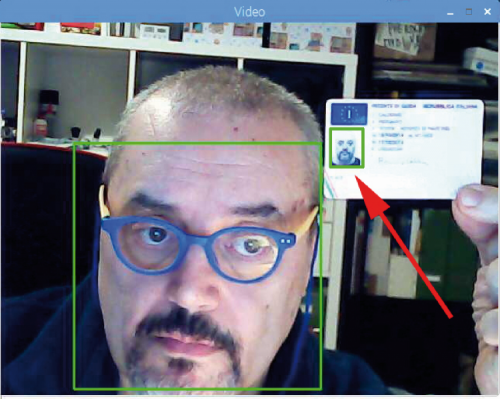
Fig. 6

 

Conclusions

Well, we can consider the discussion complete. Here, with this facial recognition project via Raspberry Pi, our journey within the OpenCV 4 library ends, although there would still be much to say and we could propose several other application examples; in the future we would like to continue publishing our experiments with OpenCV 4, so continue to follow us.

From openstore

Raspberry Pi 3 Model B+

Camera module 8 Megapixel for Raspberry Pi

 

 

Related Posts

• 

  makeITcircular 2024 content launched – Part of Maker Faire Rome 2024
  makeITcircular 2024 content launched – Part of Maker Faire Rome 2024
• 

  Application For Maker Faire Rome 2024: Deadline June 20th
  Application For Maker Faire Rome 2024: Deadline June 20th
• 

  Building a 3D Digital Clock with Arduino
  Building a 3D Digital Clock with Arduino
• 

  Creating a controller for Minecraft with realistic body movements using Arduino
  Creating a controller for Minecraft with realistic body movements using Arduino