Computer Vision with Raspberry Pi and the Camera Pi module

• Tweet
• Pin It

Let’s see how to use the Camera Pi module, a quality photo video camera, purposely designed for Raspberry PI, to acquire the  first knowledge concerning Computer Vision, to recognize colors and shapes.

Camera Pi is an excellent add-on for Raspberry Pi, to take pictures and record quality videos, with the possibility to apply a considerable range of configurations and effects. In this post we will describe how to use it to recognize specific contents within the acquired images. We may risk a definition of the Computer Vision discipline as the research and the creation of applications, distinguished by the visual capability of computers, that can be used in difficult or impractical applications for the human sight, such as the analysis of medical diagnostics images, security, or the management of autonomous vehicles. A particular sector of the Computer Vision is the Machine Vision, that has as an objective the development of applications for the quality control, the management of production processes.

In this article we will describe the basis of the Computer Vision with the tools available to almost all hobbyists: our jack of all trades, the microcomputer Raspberry Pi, Camera Pi for image acquisition (or a USB webcam), and the professional open source image processing tools, SimpleCV and Python.

 

Let’s start with introducing a couple of tools that are designed for image processing, as hinted by their names. These tools are OpenCV (Open Computer Vision) and the SimpleCV (Simple Computer Vision) framework, that allows its simplified usage with Python language. OpenCV is a specific library for Computer Vision, originally developed by Intel and released under Open Source BSD license. The library is multiplatform and can be used on the GNU/Linux, Mac OS X and Windows operating systems. The library has been designed mainly for processing images in real time, and supports the following functionalities:

• real time image capture
• video files import
• image processing (brightness, contrast, thresholds, etc.)
• object recognition (faces, bodies, etc.)
• recognition of shapes with homogenous characteristics (blob)

The immensity and versatility of the OpenCV functionalities make its utilization by the normal users quite difficult: those will find it difficult to choose and organize, as finished applications, the multitude of available “bricks” and possibilities.

Luckily, a second library comes to our aid and, whille partially limiting the functionalities of OpenCV, it makes the utilization much easier. We’re talking about SimpleCV, a framework that has been written and that is useable in Python, easy to use, that encases the functionalities of the OpenCV library and image processing algorithms into higher level “bricks” that simplify the life of the developer that wishes to create artificial vision applications, without necessarily possessing a deep knowledge of Computer Vision, such as one acquired in the most prestigious research institutes of the world. Before starting to work, let’s give some final indications on the complexity of the problems concerning Computer Vision, with some examples of what is easy and what is not easy at all, in the Computer Vision applications.

 

Let’s prepare the tools

Our vision system is composed by our Raspberry Pi, by our Camera Pi module and by the libraries that we previously described, with their dependences. Actually, Computer Vision libraries have been designed to determine and manage the vision peripherals on the USB ports, while the Camera Pi module uses a dedicated driver that manages it, by directly interfacing the CSI-2 connector.

To make up for this problem, in the Python sample programs that we present we will use the caution to acquire a photogram by means of the management controls of Camera Pi, so to load into memory the corresponding image and to process it by using the functions of the SimpleCV library.

What we have to create is an application architecture, like the one that can be seen in the scheme, with all the modules needed for the proper running of the OpenCV and SimpleCV libraries within the Raspberry Pi operating system.

 

Before starting, let’s refresh the operating system by typing in the commands from the terminal window we logged into with the “root” user.

apt-get update

apt-get upgrade

Let’s try to run Camera Pi with the command:

raspistill ‐t 5000

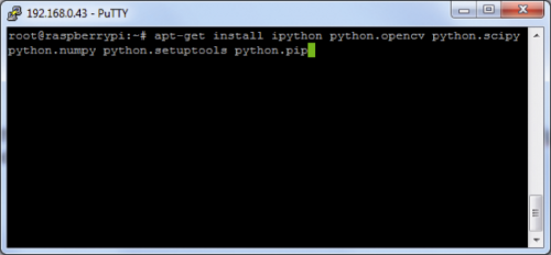
After having verified that everything works properly, we may start to install the software components of our vision system. Let’s start to install the OpenCV library, its prerequisite packages and its dependences. In particular, IPython is an “enhanced” Python interpreter, offering an interactive shell that is particularly rich in functionalities, and capable to integrate with other languages and development environments, such as SimpleCV, as we just said. Let’s install everything with the command:

apt‐get install ipython python‐opencv python‐scipy python‐numpy python‐setuptools python‐pip

 

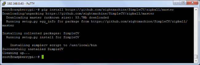
We will then move on to install SimpleCV as a Python package, and remember that pip (Python Package Index) that we just installed, is the package that allows us to manage the additional modules of the Python language:

pip install https://github.com/sightmachine/SimpleCV/zipball/master

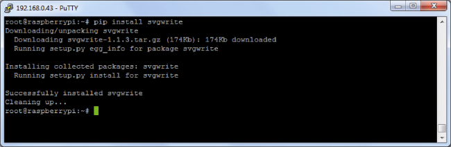
Let’s install a further dependence, needed for the running of SimpleCV, “Svgwrite”.SVgwrite deals with the management of the vectorial image format (SVG stands for Scalable Vector Graphics). Being an extension of the Python language, we install it with the pip command:

pip install svgwrite

 

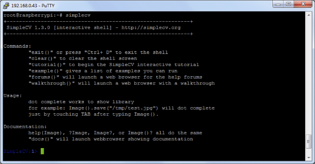
Once done with installations, we can carry out the first verifications by making use of the interactive shell supplied with SimpleCV (an equivalent function to the one available in the Python language). Let’s use the shell to verify the proper running of the OpenCV library, by typing in the command:

simplecv

 

Before starting to experiment, we should introduce, even if very briefly, the digitalization and memorization image modes. Beyond these many formats, that diversify themselves for the black and white or color mode, and by the rendering quality (number of pixels and number of colors), the images are basically represented by one or more pixel arrays, small and numerous dots that vary on the varying of size and image quality. A 640 x 480 black and white picture will be (in fact) composed by 307200 pixels (about 0,3 megapixels), each one with the size of one or more bits, that contains the shade of color that is present in the picture dot represented by the pixel itself.

A picture represented by single bit pixels will be a black (1) and white (0) picture, without shades of grey, a so-called “binarized” picture. Color pictures require a pixel matrix for each color, usually three in the RGB (red, green, blue) representation. Even here, the bit size for each pixel determines the color quality. In Table, the pixel value combinations can be seen, and they represent the main colors in the 8-bit format.

• Red: (255, 0, 0)
• Green: (0, 255, 0)
• Blue: (0, 0, 255)
• Yellow: (255, 255, 0)
• Brown: (165, 42, 42)
• Orange: (255, 165, 0)
• Black: (0, 0, 0)
• White: (255, 255, 255)

In this representation, triplets with identical values all represent shades of grey. Luckily, by using  SimpleCV it is not needed to know all the numerical representations of the colors, since the major ones can be recalled by name, as GREEN, RED, YELLOW, and so on, by typing in:

help(Color)

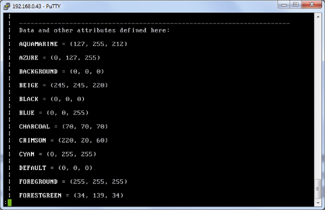
in the SimpleCV shell it is possible to obtain the list of the recognized color names.

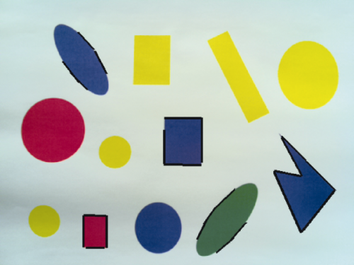
By the way, the command help(something) is the one to obtain help from SimpleCV; the help menu can be recalled with help(). Once the picture representation mode has been understood, it becomes easier to understand its processing modes. Let’s see now some easy examples, so that you can see with your own eyes, even if very briefly, the problems connected to image processing. As a reference base, we shall use a sheet upon which we have printed all the geometric format shapes, sizes and different colors.

Lighting plays a primary role, and the same goes for the distances, the camera angle, the dimensions, the contrast and the color uniformity. Do experiment. To start, in Listing 1 we see the color recognition of a specific pixel within the picture. To do so, we have to keep in mind that the elements are indexed, starting from the upper left corner of the picture. The index concerning the first pixel in the upper left corner of the picture, has a (0, 0) value. In particular, in the listing we extract the pixel value (120, 200). It is obtained by counting 120 pixels downward and 200 pixels towards the right, at about the center of the first red circle in the upper right.

 

Code 1

 

import subprocess

from SimpleCV import Image

import time

subprocess.call(“raspistill -n -w %s -h %s -o Listato1_1.bmp” % (640, 480), shell=True)

img = Image(“Listato1_1.bmp”)

img.show()

pixel = img[120, 200]

print pixel

img[120, 200] = (0,0,0)

pixel = img[120, 200]

img.save(“Listato1_2.bmp”)

print pixel

 

 

In Code, the “subprocess.call()” function allows you to launch an external process, and to wait for this to be terminated before continuing with the processing. The external process that is launched is the “raspistill” allowing you to acquire a single image and save it with the desired name. The “Image()” function loads the specified image file in a variable. The “show()” function shows the image on screen. Finally, the “img()” function allows us to access the contents of the image itself, as for reading and writing. Let’s copy the program of the Listing 1 in a file named Listato1.py in the /home folder and we will execute it with the command:

python Listato1.py

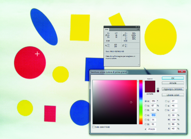
In this, and for each one of the listings that follow, we have pointed out saving of the intermediate images that are obtained during the process, so to analyze them subsequently. The pictures are then saved in the /home folder, from which they can be taken (e.g.: by using WINScp), so to open them with a visualization and/or graphic editing software. We will obtain the result that can be seen in figure, that shows the pixel value as (127, 16, 32). We can verify the correctness of the result by opening the picture with Photoshop and by visualizing the pixel value. They correspond perfectly.

 

 

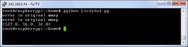
This very simple example allows us to verify in practical terms the help coming from the usage of SimpleCV, as for image processing. The img(120, 200) function does all the work for us. To set up a particular pixel with a particular color we shall use the instruction:

img[120, 200] = (0,0,0)

Obviously, we will substitute the (0, 0, 0) parameters with the R, G, B values of the color we want. This already allows us to operate on the images in the way we want, practically. In the SimpleCV library it is possible to find a lot of functions that allow to generate lines or geometric figures, to fill areas, to set up transparencies, to overwrite some test, and so on. Let’s start to describe how to recognize one or more shapes within an image. Even here we will start from a “simple” example, such as recognizing the colored areas within an image with a white background. The areas with an uniform color, for which it is possible to recognize an outline in the image processing, are defined as blobs (spots). Naturally, then, the function that recognizes the areas characterized by a color contrasting with the background, is called findBlobs(). In Code 2 we see the application of this function:

 

Code 2

 

#!/usr/bin/python

import subprocess

from SimpleCV import Image

import time

subprocess.call(“raspistill -n -w %s -h %s -o Listato2_1.png” % (640, 480), shell=True)

img = Image(“Listato2_1.png”)

img.show()

time.sleep(5)

img = img.binarize()

img.show()

time.sleep(5)

macchie = img.findBlobs()

img.save(“Listato2_2.png”)

img.show()

time.sleep(20)

 

The “binarize()” function changes the original picture into a black and white image, without shades of grey, so to “emphasize” the “spots”. Not the yellow ones, though, as they are too similar to the white background. You may try to “fix” a threshold value, one that discriminates the “spots” from the background and gives a value (0-255) to parameter of the binarize() function, e.g.: binarize(130).

 

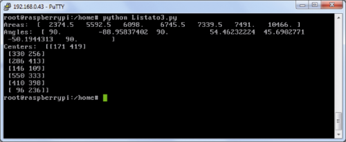
The findBlobs function, in addition to recognizing “spots”, also returns a series of information for each identified area, such as the size, the angle (direction) in respect to the x axis and the coordinates of the center of the area.

These pieces of information are very useful in robotics applications. In Code 3 we find an example of visualization of the said pieces of information. Three arrays are there highlighted: they contain the just said pieces of information. The arrays are placed in order of decreasing size of the recognized area (blob). The first “spot” to be indicated is the one of the biggest size, and then all the other ones follow.

 

Code 3

 

#!/usr/bin/python

import subprocess

from SimpleCV import Image

import time

subprocess.call(“raspistill -n -w %s -h %s -o Listato3_1.png” % (640, 480), shell=True)

img = Image(“Listato3_1.png”)

img.show()

time.sleep(5)

img = img.binarize()

img.show()

time.sleep(5)

macchie = img.findBlobs()

img.show()

time.sleep(5)

print “Areas: “, macchie.area()

print “Angles: “, macchie.angle()

print “Centers: “, macchie.coordinates()

 

 

We may now introduce the selection filters as well, to restrict the research field for possible contrasting color areas. A selection criterion is, in fact, the color. We may decide to have it to recognize only the blue color areas, and to highlight the outlines with contrasting color lines. We may do that with the Code 4 program. The reference “color” (22, 36, 75) was identified, always by using the “Photoshop” or “Gimp” method. The “colorDistance()” function takes away from the picture the pixels that represent colors that are “quite” different from the reference color, while keeping the pixels that represent colors that are “quite” similar. Once all the desidered “spots” are recognized, we highlight them with a thick black outline being three pixels wide, by means of the “draw()” function.

 

Code 4

 

#!/usr/bin/python 

import subprocess

from SimpleCV import Color, Image

import time

subprocess.call(“raspistill -n -w %s -h %s -o Listato4_1.png” % (640, 480), shell=True)

img = Image(“Listato4_1.png”)

img.show()

time.sleep(5)

colore = (22,36,75)

blue_distance = img.colorDistance(colore).invert()

blobs = blue_distance.findBlobs()

blobs.draw(color=Color.BLACK, width=4)

blue_distance.save(“Listato4_2.png”)

blue_distance.show()

time.sleep(5)

img.addDrawingLayer(blue_distance.dl())

img.save(“Listato4_3.png”)

img.show()

time.sleep(5)

 

After having launched the program, you will probably find out that the dark green ellipse is recognized as well: the color is “quite” similar to the blue, in fact. The lighting conditions may influence very much the recognition results. Once again… do experiment.

 

The next step is to recognize the outlines of a particular shape, such as lines, circles and corners. Let’s consider a segment as a sequence of points laying on a straight line, generally forming a part of an outline of the shape of a figure. The method that is used by the SimpleCV “findLine()” function is based on the Hough transform. In a few words, with this technique all the possible lines passing from the points of the bidimensional plane (that is, our picture) are analyzed. To all the points of the picture scores are assigned: they grow as they appear laying on a segment joining two points, such as the vertices of a geometric shape.

 

Code 5

 

#!/usr/bin/python

import subprocess

from SimpleCV import Color, Image

import time

subprocess.call(“raspistill -n -w %s -h %s -o Listato5_1.png” % (640, 480), shell=True)

img = Image(“Listato5_1.png”)

img.show()

time.sleep(5)

# Imposta il valore di soglia

lines = img.findLines(threshold=30)

lines.draw(color=Color.BLACK, width=4)

img.save(“Listato5_2.png”)

img.show()

time.sleep(15)

 

Let’s launch the program and probably we will find that some straight line is not recognized (maybe the sheet is not perfectly flat) while it is possible that lines “quite” straight are recognized as parts of the long “sides” of the ellipses.

 

 

Let’s use the find.Circle() function, to recognize circular figures within the picture. The function has three parameters. Canny represents the precision level (cunning) adopted by the algorithm for detecting circular shapes. The intermediate value is 100: with a higher value, the algorithm becomes more picky and recognizes a lesser amount of circles. With a lower value, the algorithm becomes friendlier and will recognize even shapes that are not perfectly circular. Thresh is the threshold level, as in the case of the straight line detection. Distance determines the minimal distance depending on which it is determined if the recognized shape consists of a single circle or more concentric circles. The rest of the instructions orders the detected circles in ascending order, depending on the area of each one. The smaller one, circles[0], is highlighted with a red outline, while all the other ones are highlighted with a black outline.

 

Code 6

 

#!/usr/bin/python

import subprocess

from SimpleCV import Color, Image

import time

subprocess.call(“raspistill -n -w %s -h %s -o Listato6_1.png” % (640, 480), shell=True)

img = Image(“Listato6_1.png”)

img.show()

time.sleep(5)

cerchi = img.findCircle(canny=250,thresh=200,distance=11)

cerchi.draw(color=Color.BLACK, width=4)

cerchi.show()

time.sleep(5)

cerchi = cerchi.sortArea()

cerchi[0].draw(color=Color.RED, width=4)

img_with_circles = img.applyLayers()

img_with_circles.save(“Listato6_2.png”)

img_with_circles.show()

time.sleep(15)

 

Launch the program and… have fun! Try to modify the parameters. Try with sheets on which you will have printed circles without filling, with the circumference of many colors, with lightings of different intensities, and so on.

To conclude with this first overview on the subject of image processing, we present the SimpleCV function that allows to read barcodes. It is obviously called “findBarcode()” and is capable to automatically recognize the type and content of the barcodes that are present in the picture. QR codes (Quick Response code) are recognized as well: they are particular bidimensional graphic codes, now very widely spread to diffuse heterogenous information, in particular towards mobile devices. A QR Code cryptogram may contain up to 7089 numeric characters or 4296 alphanumeric ones. As for the code generation, we use the Zint Barcode Studio program, an open source product that allows us to generate barcodes and QR codes of any type, and to save them as images, be it in Bitmap or vector format. Zint Barcode Studio is available for many operating systems, either with a graphical interface for “human” usage, or in library form for the program usage (Zint Barcode Generator).

For a correct interpretation of the pictures containing a barcode, we have to add the library “zbar” to the SimpleCV “store”. We may install it with the command:

apt-get install python-zbar

We have prepared a pair of barcodes, printed them on a sheet, and focused them with a video camera. The program is shown in Code 7.

 

Code 7

#!/usr/bin/python

import subprocess

from SimpleCV import Image, Barcode

import time

subprocess.call(“raspistill -n -w %s -h %s -o Listato7_3.png” % (640, 480), shell=True)

img = Image(“Listato7_3.png”)

img.show()

time.sleep(5)

# Load a one-dimensional barcode

barcode = img.findBarcode()

print barcode[0].data

 

All the examples that we described work even without the presence of a video camera. We may safely process even a series of images that have been previously acquired, or that are coming from different or remote sources. You just need to remove the instructions for the image acquisition and point the “image()” function to the path/file that contains the image you want to process.

 

Are you excited of the applications? Let us know what you’ve in mind, and stay tuned for the next update on Raspberry PI and Video Apps!… Face recognition!

 

 

Related Posts

• 

  makeITcircular 2024 content launched – Part of Maker Faire Rome 2024
  makeITcircular 2024 content launched – Part of Maker Faire Rome 2024
• 

  Application For Maker Faire Rome 2024: Deadline June 20th
  Application For Maker Faire Rome 2024: Deadline June 20th
• 

  Building a 3D Digital Clock with Arduino
  Building a 3D Digital Clock with Arduino
• 

  Creating a controller for Minecraft with realistic body movements using Arduino
  Creating a controller for Minecraft with realistic body movements using Arduino

5 Comments

1. Pingback: Machine vision with the Raspberry Pi - Artificial Intelligence Online

2. Pingback: 1wearing